Combine Multiple Conditional Formatting Rules

Topic

New Reply

I have a question for the community regarding combining conditional formatting rules.

Currently, I have 3-rules with the same formatting. They are:

=AND($A2””,AND($B20))
=AND($C2””,AND($D20))
=AND($E2””,AND($F20))

The rules are applied to rows 2-12 in columns B, D and F.

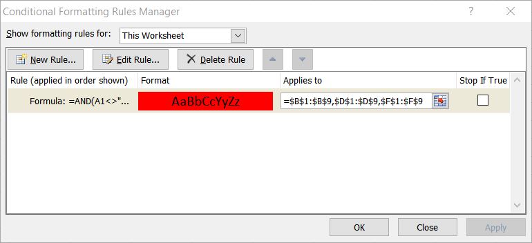
Is it possible to have a single Conditional Formatting rule that would check columns A, C and E (rows 2-12), if they are NOT BLANK, then check the values in B, D and F, if one or more ARE NOT equal to 0, apply the formatting to that particular cell?

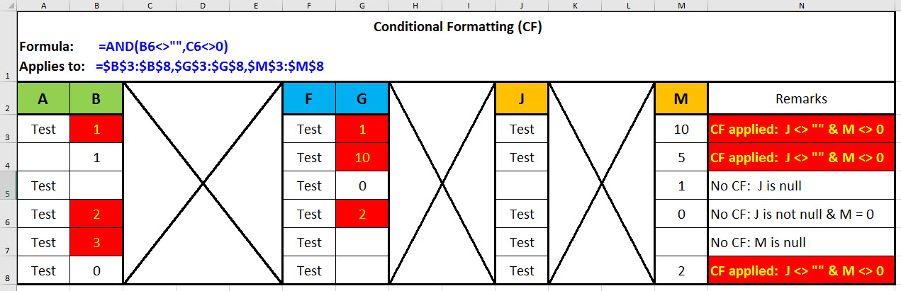
For example, if:

A2 is blank and B2 = 0 (no formatting applied to B2), C2 is NOT blank and D2 = 1 (formatting is applied to D2) and E2 is NOT blank and F2 = 0 (no formatting applied to F2). If the value of D2 is changed to 0, the formatting would disappear and if the values of B2 and/or F2 were changed to 1, the formatting would apply to those cells.

I’ve tried to combine the 3-rules into a single Conditional Formatting rule using various combinations of AND and OR statements. I’m not getting any error messaged, I am just not getting the desired results.

=AND(A2″”,AND($B20),OR(AND(C2″”,AND($D20,OR(AND(E2″”,AND($F20)))))))

Any help is greatly appreciated.

Reply | Quote

Replies

JAATR,

Is this what you want?
45418-JAATRCondFmt

The key is the range it is applied to:
[noparse]=$B$1:$B$9,$D$1:$D$9,$F$1:$F$9[/noparse]

45419-JAATRCondFmtRng

Note: You do this by highlighting the ranges above before entering the conditional formatting menus. Note: the first time I did it Excel changed the references in my formula! I had to go back in and edit the formula then it worked as expected. YMMV!

HTH :cheers:

May the Forces of good computing be with you!

RG

PowerShell & VBA Rule!
Computer Specs

Reply | Quote

RetiredGeek,

Thank you, that’s exactly what I needed. Although, to be honest I will need to study this a little to make sure I completely grasp the concept.

After I posted my message, my layout changed a little. I have inserted 5 new columns (between D and E). None of the new columns would not have any conditional formatting, so I not sure what impact this would have on the solution you provided. It’s going to be later this evening before I can test it using my new layout. I will make sure I to take a close look at the new ranges that I apply the Conditional Formatting too.

Again, thank you for your help.

Reply | Quote

Hi JAATR

As you can see from RG’s post, RG had to create a test workbook to demonstrate the solution.
Now, if you could attach a sample file for your new layout, it would then be easier for helpers to work with, and for a suggested solution to be posted back.

zeddy

Reply | Quote

RetiredGeek / zeddy,

I’ve attached the workbook. I’ve also included a screen shot. I’m sorry for the changes, I’m trying to help a family member and they think since I can turn on a computer, I’m an expert…..at this point, I think there’re set with their layout/format.

Basically, I have columns A & B and F & G applying the correct conditional formatting based on RetireedGeek’s solution. It may not be possible, but I would also like to include columns J & M into the same conditional formatting rule without creating a second rule.

45421-CF

Reply | Quote

JAATR,

You will have to create a second rule for the J:M pairing because they are not adjacent like A:B & F:G.

The same formula logic can be used just select column M then when your create the formula reference column J instead of A. The rest stays the same.

HTH :cheers:

May the Forces of good computing be with you!

RG

PowerShell & VBA Rule!
Computer Specs

Reply | Quote

I had a feeling that would be the case. I really appreciate you taking the time and effort to help me.

Reply | Quote

JAATR,

On the contrary, this can be done with one formula for the conditional formatting of Columns A-B, F-G, and J-M

Code:

The formula Rule is :
=IF(COLUMN()=2,AND($A3″”,$B30),IF(COLUMN()=7,AND($F3″”,$G30),IF(COLUMN()=13,AND($J3″”,$M30))))

And the Applied to range remains unchanged:
=$B$3:$B$8,$G$3:$G$8,$M$3:$M$8

HTH,
Maud

45430-JAATR

Reply | Quote

Maudibe,

Awesome; I cannot thank you enough. I don’t do a lot with Excel; but I know if I ever need help, someone has the answer(s). This is such a great community and I really appreciate the support I always receive.

Reply | Quote

Thanks but I saw RG do something like this a while back and its been sitting in my bag of tricks ever since!

The formula could be simplified to:

Code:

=IF(COLUMN()=13,AND($J3″”,$M30),AND(A3″”,B30))

Reply | Quote