Need to create summary of data in two-column table

Topic

New Reply

Hi folks, my XL (2010) is a bit rusty so I would appreciate a bit of a boost in the right direction, please!

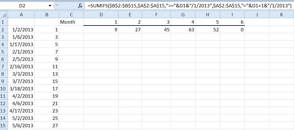
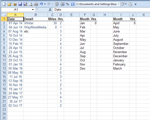
I have a list of a year’s worth of invoices with columns for the date and the number of hours for that date, and I need to get a summary of the number of hours per month, in the form of a two-column table with the month and the numbers of hours for that month.

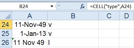
I’m presuming I therefore need to have something that can identify the month part of the date and, where this matches the month in the results table, add the number of hours together in the corresponding total hours cell. Main problems I’m having are getting it to identify the month out of the date in each case, and getting it to add up all the entries that match the month.

I know I’m rusty because I remember using something similar with vlookup and possible multiple entries that need totalling, but I can’t remember for the life of me how I did it (and I’m not in the job that was for any more (haven’t been for a couple of years or so) so I can’t look back and check, either!).

Any assistance would be greatly appreciated!

Many thanks!

Reply | Quote

Replies

Beryl,

Here’s one possible solution. I’m not sure it is the best one but it’s the best I can come up with the moment.
[noparse]=SUMIFS($B$2:$B$15,$A$2:$A$15,”>=”&D1&”/1/2013″,$A$2:$A$15,”<"&D1+1&"/1/2013")[/noparse]
36811-Beryl
Note: this formula can be copied across the column but you will have to adjust the dates for the December entry changing the ending date to reflect the next year and the month to reflect 1 vs 13.

Of course if you are willing to add a column to your worksheet you could use the formula [noparse]=Month(A2)[/noparse] and copy it down the column. You could then use a Pivot Table to do all the work for you. HTH :cheers:

Test File: 36812-Beryl

May the Forces of good computing be with you!

RG

PowerShell & VBA Rule!
Computer Specs

Reply | Quote

Hi RG, thanks for this but I must admit I was hoping for something that didn’t include the year – and my layout is per the attached, sorry should have done that in the first place. I can live with the shortened versions of the months (Jan, Feb, etc) in both original and results but would really prefer to have shortened ones in original and full length in results – that’s why I wanted something that had XL recognising that they were months!

36815-woodys

In fact I have just tried to apply your suggestion but it didn’t work – I’ve a feeling it relies on the fact that your months are displayed as numbers, and of course mine aren’t.

Thanks for the suggestion, though.

Reply | Quote

Hi Beryl

..have a look at the attached file.
I added some columns to simplify things.
The formulas are now simpler.

If you have any questions, please ask.

zeddy

Reply | Quote

Beryl

This can be done simply with a Pivot Table. The steps to do it are:
1. Select the range A1 to D22 and go to Insert > Pivot Table
2. In the Create PivotTable dialog, choose to place the pivot on either a new worksheet or somewhere like ‘Sheet1!$L$1’ and click OK
3. In the PivotTable Task Pane which appears, drag Date into the Row Labels section and Hrs into the Values section.
4. Now right click on the first column of the pivot table itself and choose Group… and select by Months

Reply | Quote

Beryl,

From looking at your data I suspect that you may not have dates (which are values) but rather text that look like dates. I’m using Excel 2010 and it is impossible to enter dates to look like you have them, unless you have applied a custom format of some kind. If you notice in the file Zeddy provided for you all the dates have dashes in them because they are values (date values). You can test this with the Cell function:
36818-Beryl
Note: Cell returns a “b” if the referenced cell is blank, “v” if there is a value/formula in the referenced cell and “l”, for label, if there is anything else as shown above. You’ll notice “dates” as you have them shown in your posting return “l” and thus can’t be used to calculate using either zeddy’s or my solutions. Please check this out to see if this is the case. HTH :cheers:

Update: I just noticed that you posted a file and it does have the dashes and they are values. I don’t know why they don’t show in the screen capture? I’ll leave this post because the information may be of use to others. :cheers:

May the Forces of good computing be with you!

RG

PowerShell & VBA Rule!
Computer Specs

Reply | Quote

RG,

That’s one those handy little tools that always gets lost in the shuffle! Just made a short macro of it and added it to my personal

Reply | Quote

Maud,

Care to post the macro? I’d love to see it. :cheers:

May the Forces of good computing be with you!

RG

PowerShell & VBA Rule!
Computer Specs

Reply | Quote

Okay, thanks again RG and Zeddy – I’ve got something usable now that’s *almost* exactly what I wanted! I discovered that I don’t need to add an extra column to the results table, if I get the list of month labels by entering them as dates (doesn’t matter what the date is as long as the month is right in each case) and formatting them as “mmmm” – that is, I put “1 1 1” in the cell for January (without the quotes, of course), “2 2 2” for February, etc. Having done that, Zeddy’s formula can be slightly modified to:

=SUMIF($E:$E,MONTH(L2),$D:$D)

And it works perfectly. I still can’t work out how to get XL to pick the month out of the date in column A rather than have to add column E, and have therefore had to add that column but hidden so it doesn’t interfere with the layout of the form.

One other thing to note, if you want to use this, or a variation of it – the extra (hidden) column can’t just be “=Month(A1)” all the way down as for some reason XL reads a blank cell as “1”, which would throw all the January figures, so I ended up using “=if(A1″”,Month(A1),””)”. That’s if, as I am, you’re setting up a ‘master’ that will get filled in over the year, and don’t know exactly how many rows it’ll be yet, not to mention will be blanking and reusing it for next year. I’ve assumed a max of 200 and filled in my formalae down that far.

Once again, many thanks, everyone – although if anyone does know how to get XL to extract the month from the date without having to use an extra column, please do say so! That would make it just perfect!

:clapping:

Reply | Quote

RG,

Here is my UDF equivalent of your Cell function in VBA

36822-CellType1

Code:

Public Function CellType(rng As Range)
CellType = VarType(rng)
End Function

Reply | Quote

Maud,

Thanks! That’s even better than CellType since it returns more granular information.

HTH :cheers:

May the Forces of good computing be with you!

RG

PowerShell & VBA Rule!
Computer Specs

Reply | Quote