Trying to Understand

Topic

New Reply

I have searched far and wide for a suitable explaination without much success so hoping I can find the answer here.
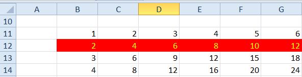
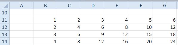
With conditional formatting assuming my work area is B11 to R41, when creating a formula I would write $B11=2 then in the box to cover where the formula is valid it would be =$B$11:$R$41

What I would like to know is if I enter a “2” in for example B33 then the formatting works for that row, which part of the formula is doing this? How does B33 relate to just that row for example and why is it not defined in the formula box ( it just refers to =$B11=2?

Thanks

Alan

Reply | Quote

Replies

Allen,

The behavior you see is cause by the use of the MIXED reference in your formula, e.g. $B11.
The B part is FIXED by the $ however the 11 (row) part is not so it will change to operate for each row.

Per your parameters: =$B11=2
37106-cf1
Notice how it operates for row 12 with a value of 2 in B12.

If you change the formula to =$B$11=2
37107-cf2
Notice how now since the reference is fixed on both parts (or an Absolute Reference in Excel speak) nothing is formatted because $b$11 is NOT equal to 2. However if $B$11 is set to 2 all cells will be formatted.
37108-cf3

HTH :cheers:

May the Forces of good computing be with you!

RG

PowerShell & VBA Rule!
Computer Specs

Reply | Quote

To expand on RG’s comments. It is about Absolute vs relative references in cells. One way to look at it would be to imagine that you would copy the formula:
=$B11=2

into the range
=$B$11:$R$41

and imagine what the formulas would be [ignoring that they would be circular references]

Since the Column B is Absolute [=preceded by a dollar sign($B)] but the row is relative [not preceded by a dollar sign] in the cells in row 11 B11:R11] the formula would amount to:
=B11=2

So for any cell in row11, if B would be 2 they would all be “TRUE” and meet the condition.

That is the same for each row. Row 40 for example in Cells B40:R40 would all have:
=B40=2

So again they are all comparing to the value in col B for that row.

Each cell can have 1 of 4 abs/rel combinations [Tip: when entering formulas the key toggles through the 4 possibilities:]
=B11
=$B$11
=B$11
=$B11
If you had used B11 and copied the [=B11=2] into the B11:R41 cells, the cond format would be true when a particular cell had the value of 2
If you had used [=$B$11=2] into the B11:R41 cells, the cond format would be true for all the cells when B11 equals 2
If you had used [=B$11=2] into the B11:R41 cells, the cond format would be true for any cells in the column when the value in row 11 equals 2
And to reiterate your example, when you had used [=$B11=2] into the B11:R41 cells, the cond format would be true for any cells in the row when the value in Col B equals 2

Hope this helps,
Steve

Reply | Quote

Thankyou both very much, that is easier to understand than the references I found on the net.

Alan

Reply | Quote