variable based on total

Topic

New Reply

See attached example.
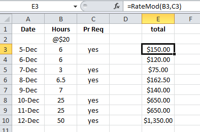
Hourly rate is $20. Number of hours is column B. Hourly rate is modified when “Pr Req” column [C] = “yes”. The rate modification varies by the total of column “B” when column C is “yes”. In example, Row 3,5,6,8,9,10, Column C =yes. The totals in column E for each of these rows must include the rate increase in the table below. So, rows 3,5,6 would be increased by $5/hr [to $25/hr], row 8 by $6, row 9 by $7, etc.

Rate Table:
Increase base by these amounts when the total hours in column B equals:
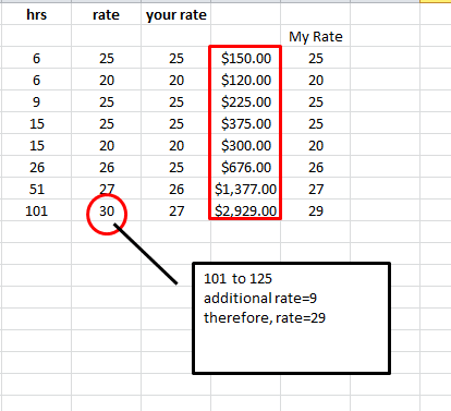
HRs= 0-25 = $5
25-50=$6
51-75=$7
76-100=$8
100-150=$10

So, if the total of column “B”, with corresponding “yes” in column C =54, then the base rate per hour of $20 is increased to $27/hr.

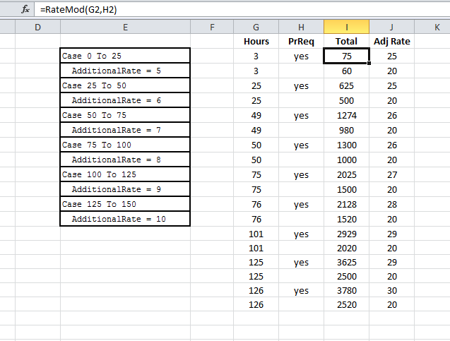
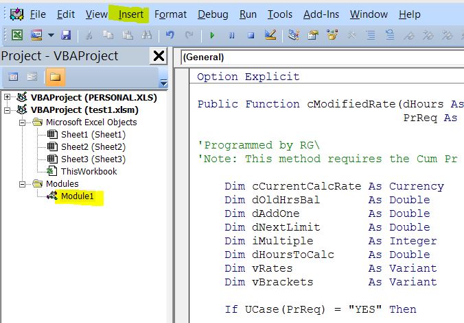
My solution is somewhat crude. I have a column G that totals the designated rows for increase in column “B” and then use this formula:
=G4*IF(G4<=25,5,IF(G4=26,6,IF(G4<51,6,IF(G4=51,7,IF(G4<76,7,IF(G4=76,8,IF(G4<101,8,IF(G4=101,10,IF(G4<126,10)))))))))

How can I do this without the extra column G [of totals] and can I simplify the formula?
Thanks

Reply | Quote

Replies

In E3:
=B3*(20+IF(C3=”yes”,INDEX({5,6,7,8,10},MATCH(SUMIF($C$3:C3,”yes”,$B$3:B3),{0,25,51,76,100})),0))

Copy down the column. It may be more efficient to create a rate table of the sums and increase and just do a vlookup, instead of having the array in the formula.

Steve

Steve

Reply | Quote

Thanks sdckpr.
How would I do the rate table you suggested?

Reply | Quote

How would I do the rate table you suggested?

For example, in G1:G5, enter the min for each rate. From your example: 0,25,51,76,100 respectively. Then in H1:H5 enter the add’t rate: 5,6,7,8,10. Then you can use the formula in C3:
=B3*(20+IF(C3=”yes”,VLOOKUP(SUMIF($C$3:C3,”yes”,$B$3:B3),$G$1:$H$5,2),0))

To lookup the rate based on the total in that table. The table could be placed elsewhere or on another sheet if desired.

Steve

Reply | Quote

This can also be done as a User Defined Function (UDF): =RateMod(Hours, PrReq)

Enter in cell E3 =RateMod(B3,C3) and then copy down. This assumes that the upper limit values of each bracket (ex. 25, which also equals the lower limit values of the next bracket) references the next bracket up. This can be change by reversing the order of the Case statements.

There are no extra columns and the formula =RateMod(B3,C3) is about as simple as it gets. Paste the code in a standard module.

HTH,
Maud

35862-Example1

Code:

Public Function RateMod(Hours As Double, PrReq As String) As Currency
Dim AdditionalRate As Currency
    If UCase(PrReq) = “YES” Then
        Select Case Hours
            Case 0 To 25
                AdditionalRate = 5
            Case 25 To 50
                AdditionalRate = 6
            Case 50 To 75
                AdditionalRate = 7
            Case 75 To 100
                AdditionalRate = 8
            Case 100 To 150
                AdditionalRate = 10
        End Select
    Else: AdditionalRate = 0
    End If
RateMod = (20 + AdditionalRate) * Hours
End Function

Reply | Quote

Maudibe,
Thanks. Attached is a slight modification of your example. I added another breakdown I forgot. Both your example and mine become incorrect over 25 hours.
In my example [example_Revised #2] Col G is total hrs to be counted, col H is the correct rate, col I is your/my rate. I also modified your “Case 25 To 50” to “Case 26 To 50” etc, thinking that was the problem. None gave correct returns over 25 hrs.

Reply | Quote

Skipro,

Rate Table:
Increase base by these amounts when the total hours in column B equals:
HRs= 0-25 = $5
25-50=$6
51-75=$7
76-100=$8
100-150=$10

You need to correct your rate table as according to this table 25 hours is both +$5 & +$6 etc.
So what you need would be something like this:
<26 hrs = 5
<51 hrs = 6
etc.
Or
<25 hrs = 5
<50 hrs = 6

Which do you want?

If it is the first one this code:

Code:

Public Function cModifiedRate(Hours As Double, PrReq As String) As Currency

    Dim cAdditionalRate As Currency
    
    If UCase(PrReq) = "YES" Then
        Select Case Hours
            Case Is < 26
                cAdditionalRate = 5
             Case Is < 51
                cAdditionalRate = 6
            Case Is < 76
                cAdditionalRate = 7
            Case Is < 101
                cAdditionalRate = 8
           Case Is < 126
                cAdditionalRate = 9
           Case Is < 151
                cAdditionalRate = 10
         End Select
    Else
      cAdditionalRate = 0
    End If
    
  cModifiedRate = (20 + cAdditionalRate) * Hours
  
End Function   'cModifiedRate

Otherwise reduce each test number by 1.

HTH :cheers:

May the Forces of good computing be with you!

RG

PowerShell & VBA Rule!
Computer Specs

Reply | Quote

Neither of these work. Get same results. They do not add the total numbers associated with “yes” to get the proper rate. They get same result for every “25” entered. They should increase rate.
See attached examples for both.

Reply | Quote

You need to correct your rate table as according to this table 25 hours is both +$5 & +$6 etc.

RG,

Actually you don’t need to change them. Just like your example, 25 will satisfy all case statements but only the first true statement is processes. If case=0-25 and 25-50, only the first case statement in my code will be processed as well.

This assumes that the upper limit values of each bracket (ex. 25, which also equals the lower limit values of the next bracket) references the next bracket up.

Skipro,

As I stated in my above post, the code in the workbook referenced the higher bracket, I now know you want 25, 50, etc., to reference the lower bracket. In your example rev2, you quoted 101 hours as a rate 0f 30 but in the code, you modified the line:

Case 101 To 125
AdditionalRate = 9

Therefore, the rate should be 29 not 30 and the total of $2,929.00

Code:

Public Function RateMod(Hours As Double, PrReq As String) As Currency
Dim AdditionalRate As Currency
    If UCase(PrReq) = “YES” Then
        Select Case Hours
            Case 0 To 25
                AdditionalRate = 5
            Case 25 To 50
                AdditionalRate = 6
            Case 50 To 75
                AdditionalRate = 7
            Case 75 To 100
                AdditionalRate = 8
            Case 100 To 125
                AdditionalRate = 9
            Case 125 To 150
                AdditionalRate = 10
        End Select
    Else: AdditionalRate = 0
    End If
RateMod = (20 + AdditionalRate) * Hours
End Function

Attached is the modified sheet that corrects everything.

35871-RateMod1

Maud

Reply | Quote

Skipro,

I have run a check on various scenarios and all appears correct. The reason I am leaving 25, 50, 75, etc., in more that one case statement is that if there are 25.5 hours, or example, it will be included (25 to 50)

35873-RateMod2

Maud

Reply | Quote

Maudibe,
Figured out we are going in different directions. Yes, you are correct, your method is correct for that row. That is where I did not explain well enough. The rate is dependent on the TOTAL of the hours, not just that row.

If the first row of hours [B3] is 24 hrs, the rate is for those 24 hours is 25. If the second row [B4] is 24 hours, the rate for the 1st hr is 25, for hour #25, the rate for the other 23 hrs is 26, for hours # 26 to 48. If the third row [B5] is 50 hours, the rate for the 1st 2 hours is 26 for hours 49 & 50, the rate for the next 25 hours is 27 for hours 51-75 and the last 23 hours rate is 28 for hours #76 to 98. I hope this is clear.

I am attaching an example I hope explains this adequately.

Reply | Quote

Maud,

This assumes that the upper limit values of each bracket (ex. 25, which also equals the lower limit values of the next bracket) references the next bracket up.

That’s exactly what I was trying to get the OP to clarify. As the rates stood you need to assume and we all know about that.

Yes, the Select construct will execute only the first Case matched but here again it is better to have clarity IMHO as to where the limits are.

And as we both just found out from the previous post clarity of requirements are sometimes hard to find! :cheers:

May the Forces of good computing be with you!

RG

PowerShell & VBA Rule!
Computer Specs

Reply | Quote

SkiPro,

I think (on occasion) that this is what you are after.

Code:

Option Explicit

Public Function cModifiedRate(dHours As Double, dPrevCumHrs As Double, _
                              PrReq As String) As Currency

    Dim cCurrentCalcRate As Currency
    Dim dOldHrsBal       As Double
    Dim dAddOne          As Double
    Dim dNextLimit       As Double
    Dim iMultiple        As Integer
    Dim dHoursToCalc     As Double
    
    If UCase(PrReq) = "YES" Then
    
      iMultiple = dPrevCumHrs / 25  'Note: I want the integer value only!
      dAddOne = IIf(dPrevCumHrs  25 = 0, 1, 0)
      cCurrentCalcRate = iMultiple + 5 + dAddOne + 20 'Note: Hard coded value
      dNextLimit = (iMultiple + 1) * 25
      
      Do
      
        If (dHours + dPrevCumHrs) <= dNextLimit Then
          cModifiedRate = cModifiedRate + (dHours * cCurrentCalcRate)
          dHours = 0
      Debug.Print cCurrentCalcRate, dNextLimit, cModifiedRate
        Else
          dHoursToCalc = dNextLimit - dPrevCumHrs
          cModifiedRate = cModifiedRate + dHoursToCalc * cCurrentCalcRate
          dPrevCumHrs = dNextLimit
          dNextLimit = dNextLimit + 25
          cCurrentCalcRate = cCurrentCalcRate + 1
          dHours = dHours - dHoursToCalc
      Debug.Print cCurrentCalcRate, dNextLimit, cModifiedRate
        End If
        
      Loop Until dHours = 0
      
   Else
     cModifiedRate = dHours * 20
   End If
  
End Function   'cModifiedRate

Results look like this with my notations.
35878-SkiPro
Note the addition of the Cum PR column and it's formula as shown in the formula bar.
You need to type this in D3 then fill down.
I'd also recommend that you change B2 to be a value and then adjust the macro to reference B2 which will make it much easier to change the Base Rate. HTH :cheers:

May the Forces of good computing be with you!

RG

PowerShell & VBA Rule!
Computer Specs

Reply | Quote

Here is a UDF that I came up with, if you don’t want a formula

Code:

Option Explicit
Function RateMod(rSubTotal As Range, sPrReq As String) As Double
  Dim dSubtotal As Double
  Dim dHours As Double
  Dim dRate As Double
  Dim vHours As Variant
  Dim vAdd As Variant
  Dim x As Integer

  'Change these as desired
  dRate = 20
  vHours = Array(0, 25, 51, 76, 100)
  vAdd = Array(5, 6, 7, 8, 10)
  dSubtotal = Application.WorksheetFunction.Sum(rSubTotal)
  dHours = rSubTotal(rSubTotal.Count)
  
  If UCase(sPrReq) = "YES" Then
    x = Application.WorksheetFunction.Match(dSubtotal, vHours)
    dRate = dRate + vAdd(x - 1)
  Else
    dRate = dRate
  End If
  RateMod = dRate * dHours
End Function

Add it to a module and then in E3 you can use something like:
=ratemod($B$3:B3,C3)

And copy it down the column.
Steve

Reply | Quote

skipro,

You have a lot of choices here:

Here is a macro that does not require you to add any formulas on the sheet to do the calculations. I have provided you with the breakdown. You can continue to add as many values to columns 2 and 3

HTH,
Maud

35880-RateMod3

Code:

Public Sub RateModification()
[COLOR=”#008000″]’————————————-
‘DECLARE AND SET VARIABLES[/COLOR]
LastRow = ActiveSheet.Cells(Rows.Count, 2).End(xlUp).Row
Hours = 0
Subtotal = 0
[COLOR=”#008000″]’————————————-
‘CALCULATE HOURS, BRACKETS, AND TOTALS[/COLOR]
For I = 3 To LastRow
    If UCase(Cells(I, 3)) = “YES” Then [COLOR=”#008000″]’PR REQ VALUES[/COLOR]
        Hours = Hours + Cells(I, 2)
        Select Case Hours
            Case 0 To 25
                Total = Hours * 25
            Case 25 To 50
                Total = (625) + ((Hours – 25) * 26)
            Case 50 To 75
                Total = (1275) + ((Hours – 50) * 27)
            Case 75 To 100
                Total = (1950) + ((Hours – 75) * 28)
            Case 100 To 125
                Total = (2650) + ((Hours – 100) * 29)
            Case 125 To 150
                Total = (3375) + ((Hours – 125) * 30)
        End Select
        Cells(I, 5) = Total – Subtotal
        Subtotal = Total
        Else:  [COLOR=”#008000″]’NON PR REQ VALUES[/COLOR]
            Cells(I, 5) = Cells(I, 2) * 20
            Cells(I, 6) = Cells(I, 2)
    End If
Next I
End Sub

Reply | Quote

Need revision help. The “powers to be” have revised their system. The good news is that the changes are minimal and make the original complex problem easier. The Rate tables are beyond my knowledge so I am unable to do the modifications. I am assuming using Rate tables is the more optimal approach, if not please let me know. I realize some of this can be done with simple formulas but not sure if this is the best way to go or if the easier stuff should be incorporated into the scripts.

I now have 2 rate tables to incorporate. Can the two be kept separate in the scripting to make it easier for me to understand and then change as future needs change?

Attached is an example of the new requirements. See inserted comments for origin of amounts.
When Pr Req totals 26, as shown in column “I” [not the sum of entries in “I”], then column “M” would show $6.00, from V6. I do not want to have to put 23 more entries to show this. See row 14. I am showing “I” = 26 for example only.

1) In the ORIGINAL SPREADSHEET “Pr Req” rate was based on the product of total number of “yes” and the hrs associated with them, column “D”, “Cum Pr”. A “yes” associated with 6 hrs equaled 6. Now the rate is based only on the number of “yes” and not the product of hrs and “yes”. A “yes”, associated with 6 hrs, equals 1, not 6, as in the original design. I need to remove the multiplication factor. The number of “Pr Req” is still cumulative and would increase by one “1” for each additional “yes”.
I need the total number of Pr Req [at that time/row] in column “I”. This number will correspond to Column “U” in rate table for that instance or row only.

2) In the original spreadsheet the pay total [columns E to G] is automatically calculated by the scripts. I need to break this down to “Pr Req rate added to base rate per hr” from “column “V” in rate table” placed in [column “M”].
“Pr Req rate increase per Hr” [column “V”] needs to be indicated in column “M”.
EX: If “yes” in column “H” corresponds to a total of “0” to “25” “yes”s, then $5.00 would be in column “M” associated with those “yes” rows.
B} I need the total added rate [“Pr Req rate added to base rate per hr” TIMES “Hrs”] in column “N”.
The product of “M” times “Hrs”, column “D”, in column “N”.

3) Column “I”: When column “C” is GRP, then “I” = “GRP”, not “0”.

2) Additional rate table is “GRP Hd Cnt” [columns R/S, rows 5-12]
Column “G” is number associated with column “R” in rate table. Column “S” is addition rate per Hr. The rate increase from column “S” goes in column “K”
Ex: “G” = 5, then place $1.50, from column “S”, in column “K”, regardless of the total number of previous “G”s.
This is NOT cumlative, but on a case [or entry] by case [or entry] basis.
B} I need the product of “K” times “Hrs”, column “D”, in column “L”.

3) Is it possible to use the “rate tables” [R/S 5:12] as variables in the scripting so I could change them instead of the scripts?

Reply | Quote

Interesting comparison of results from each solution using same data.

35885-RateMod4

Reply | Quote

Maud,

:thewave:

Nice work! I’ve been racking my brain on this all day and the edge cases just kept giving me headaches.

If I may here’s a slight change to make your code conform to the OPs original table of rates. There is no $29 rate it jumps from 28 to 30 there is also no rate for more than 150 hours so I would assume it doesn’t change or the situation hasn’t yet been seen. In either case how about?

Code:

        Select Case Hours
            Case 0 To 25
                Total = Hours * 25
            Case 25 To 50
                Total = (625) + ((Hours - 25) * 26)
            Case 50 To 75
                Total = (1275) + ((Hours - 50) * 27)
            Case 75 To 100
                Total = (1950) + ((Hours - 75) * 28)
            Case Else
                Total = (2650) + ((Hours - 100) * 30)
        End Select

HTH :cheers:

May the Forces of good computing be with you!

RG

PowerShell & VBA Rule!
Computer Specs

Reply | Quote

Could you attach your spreadsheet? The numbers I get from my formulas and/or UDF do not match what you report for me (I get: 150, 120, 75, 162.5, 140, 675, 700, 1500, respectively). I presume you have entered the range incorrectly in the UDF.

Steve

Reply | Quote

Steve,

Here’s what I’ve been working with which has Maud’s, Yours, and Mine (luckily we all used different names). See row 10 and my explanation of how it should be calculated as I understand. You’ll notice only Maud has it right. I did at one point but others it messed up other lines.

HTH :cheers:

May the Forces of good computing be with you!

RG

PowerShell & VBA Rule!
Computer Specs

Reply | Quote

In my UDF I failed to subtotal just the YES values. How is this:

Code:

Function RateMod(rSubTotal As Range, rPrReq As Range) As Double
  Dim dSubtotal As Double
  Dim dHours As Double
  Dim dRate As Double
  Dim vHours As Variant
  Dim vAdd As Variant
  Dim x As Integer

  'Change these as desired
  dRate = 20
  vHours = Array(0, 25, 51, 76, 100)
  vAdd = Array(5, 6, 7, 8, 10)
  dSubtotal = Application.WorksheetFunction.SumIf(rPrReq, "yes", rSubTotal)
  dHours = rSubTotal(rSubTotal.Count)
  
  If UCase(rPrReq(rSubTotal.Count)) = "YES" Then
    x = Application.WorksheetFunction.Match(dSubtotal, vHours)
    dRate = dRate + vAdd(x - 1)
  Else
    dRate = dRate
  End If
  RateMod = dRate * dHours
End Function

This is called with:
=RateMod($B$3:B9,$C$3:C9)

I get diff values for rows 9, 10, 11. I get 675, 1500, 3000 (rates, 27, 30, 30) instead of Maudibe’s rates of 26.04, 27.56, and 30.

Steve

Reply | Quote

Steve,

You are calculating all hours on a line at the same rate. If I’m understanding the OPs requirements you need to figure how many hours to apply to each rate based on past history thus the breakdown in my post and Maud’s posts. Of course this is ASSUMING we have the correct interpretation. :cheers:

May the Forces of good computing be with you!

RG

PowerShell & VBA Rule!
Computer Specs

Reply | Quote

I assume the breakdown on each line is based on the subtotal of all the previous YES. I use the SUMIF so no intermediate calculation is required (which was one of the requests).

But I agree we need to wait for the OP to chime in on which methodology is correct.

Steve

Reply | Quote

RG,

in post #5 Skipro adds a missing bracket of $29. In post #10, the OP makes it clear how the hours are calculated.

Maud

Reply | Quote

RG,

in post #5 Skipro adds a missing bracket of $29.

Maud

Maud,

Oops! I didn’t open that version so I missed that. This thread takes me back to my working days where we’d spend months hashing out requirements before we ever wrote a line of code. It was arduous but when you actually started to write the code it was clear what needed to be done. Of course after you had it coded there was the inevitable “that’s not what I meant” and/or “oh I forgot to mentioin”. :cheers:

May the Forces of good computing be with you!

RG

PowerShell & VBA Rule!
Computer Specs

Reply | Quote

I misunderstood completely. Here is a modified UDF

Code:

Option Explicit
Function RateMod(rSubTotal As Range, rPrReq As Range) As Double
  Dim dSubtotal As Double
  Dim dPrevSub As Double
  Dim dCurrHours As Double
  Dim vHours As Variant
  Dim vRate As Variant
  Dim vInter As Variant
  Dim x As Integer
  Dim dRate As Double

  'Change these as desired
  dRate = 20
  vHours = Array(0, 25, 50, 75, 100)
  vRate = Array(25, 26, 27, 28, 30)
  
  'Calc variables
  dSubtotal = Application.WorksheetFunction.SumIf(rPrReq, "yes", rSubTotal)
  dCurrHours = rSubTotal(rSubTotal.Count)
  dPrevSub = dSubtotal - dCurrHours
  'Calc intermediate array
  ReDim vInter(0 To UBound(vHours))
  vInter(0) = 0
  For x = 1 To UBound(vHours)
    vInter(x) = vInter(x - 1) + (vHours(x) - vHours(x - 1)) * vRate(x - 1)
  Next
  If UCase(rPrReq(rSubTotal.Count)) = "YES" Then
    'Total for Prev Subtotal
    x = Application.WorksheetFunction.Match(dPrevSub, vHours) - 1
    RateMod = vInter(x) + (dPrevSub - vHours(x)) * vRate(x)
    'Incremantal increase for Curr Hours
    x = Application.WorksheetFunction.Match(dSubtotal, vHours) - 1
    'curr subtotal - prev subtotal
    RateMod = vInter(x) + (dSubtotal - vHours(x)) * vRate(x) - RateMod
  Else ' Not a Yes, just use std rate
    RateMod = dCurrHours * dRate
  End If
End Function

In row 3 it wojuld be called with something like:
=RateMod($B$3:B3,$C$3:C3)

This is a function and does not use the CASE or IF, but a lookup Array that is created, so it should be easier to maintain if the values change or more increments are needed.

Steve

Reply | Quote

A modification like that, can be done by changing the lines:

Code:

  vHours = Array(0, 25, 50, 75, 100)
  vRate = Array(25, 26, 27, 28, 30)

to

Code:

  vHours = Array(0, 25, 50, 75, 100, 125)
  vRate = Array(25, 26, 27, 28, 29, 30)

This allows the borders and increments to be changed easily. If they will be regular increments as they are now, it could be calculated as a series, bu keeping the array allows for non-regular changes (eg like using IRS tax Tables).

Steve

Reply | Quote

Guys,
Amazing amount of work going into this for me. **Thanks**
Much of this is over my head but let me try to clarify things.
1) I originally assumed a $9 rate, but later realized it jump from $8 to $10.

2) Base rate of $20 [which may change in time] which is augmented or increased by the rate on the rate table [which also may change in time]
It may be helpful to have a cell containing the “base rate” so a modification could be made to this cell instead of changing script or formulas.

3) Rephrasing to add clarity:
1st ’25’ – $5
2nd ’25’ – $6
3rd ’25’ – $7
4th ’25’ – $8
5th ’25’ – $10
etc
Rate is on accumulative or total numbers.

4) I did not include the entire rate table, figuring I could add/extrapolate later.
Entire rate table is:
0-25 $5
26-50 $6
51-75 $7
76-100 $8
101-125 $10
126-150 $12
151-175 $14
176-200 $16
200+ $18

I hope this helps.

Because you have lost me a while back with your replies/solutions, does this info change anything, other then the additional “base rate” cell idea?
Which of the replies works as needed or is this still a work in progress?
Again, thank you for all the work you have given this.

Oh, Merry Christmas.

Reply | Quote

SkiPro,

Ok, here’s a worksheet with 2 solutions that work (at least according to what Maud & I think you want. Steve has a different interpretation of how to calculate the rate for a given set of hours. The way Maud & I see it if there are 99 cumulative hours so far and the next row has 27 hours to charge 1 hour would be charged at $28, 24 @ 30, and 1 @ 32. If this is correct either of the two solutions (Maud’s or Mine will work). If this is an incorrect interpretation you may want the solution Steve has provided which would calculate all 27 hours at a single rate.

@Steve: I borrowed your idea using the variant arrays for the rates/brackets made my code a lot simpler…THANKS!

BTW: I added a named range for the Base Rate so it can simply be changed in the workbook.

HTH :cheers:

May the Forces of good computing be with you!

RG

PowerShell & VBA Rule!
Computer Specs

Reply | Quote

Retired Geek,
You did not put in my latest code and to call it, use:
=RateMod($B$3:B3,$C$3:C3)
Currently my method matches your values

Skipro,
I think you should post a workbook with some example calcs and the correct values, especially those with subtotals on the borders. Also are there no part hours? What happens between eg 25 and 26 or 75 and 76, etc.

Steve

Reply | Quote

Steve,

Sorry for not grabbing your latest code. I’ve included it in the file below and I modified the array to include the latest rates provided by OP. Your code now comes up with the same answers with the exception of the last two rows (with large numbers of hours spanning several rates). I looked but couldn’t see the problem so I’ll let you fix it. :cheers:

May the Forces of good computing be with you!

RG

PowerShell & VBA Rule!
Computer Specs

Reply | Quote

Your vRate was inaccurate. You had values of:
vRate = Array(25, 26, 27, 28, 29, 30, 32, 34, 26, 38, 38)
It should have been (there is no 29 and the 26 should have been 36):
vRate = Array(25, 26, 27, 28, 30, 32, 34, 36, 38, 38)

Also the double 38 is not needed since the rate does not change at 1000. You can simply use:
vHours = Array(0, 25, 50, 75, 100, 125, 150, 175, 200)
vRate = Array(25, 26, 27, 28, 30, 32, 34, 36, 38)

With that change the numbers match.

Steve

Reply | Quote

Steve,

Sorry once again! I copied the items from your last post but that was before the OPs last rate update and I didn’t proof. :angry:

So here’s the final sheet with 3 different methodologies that all accomplish the same task. Ain’t computers wonderful.

@Steve: I modified your code and arrays to use the BaseRate stored on the Worksheet per OP req.

Note: Steve’s method is the only one that requires nothing other than the VBA code! No supporting columns or buttons needed. HTH :cheers:

May the Forces of good computing be with you!

RG

PowerShell & VBA Rule!
Computer Specs

Reply | Quote

On the contrary, even UDF’s are dependent upon worksheet formulas or other code to call it. The only true way is through an event routine.

Reply | Quote

I think what RG meant was that his required an intermediate calculation column, while mine does not (which is what the user asked about) and yours is not a funtion (which both RGs and mine are) so would require something to trigger your code to run. Yours also needs to work through all the dataset. My function only requires the current subtotal with YES and the amount of the new amount added, it requiures no other preliminary values (the preliminary values are only used to calc the current subtotal).

Steve

Reply | Quote

Folks,
Thanks, but I cannot get RetiredGeeks last example to work when I make a spreadsheet.
See attached example.

Reply | Quote

SkiPro,

The problem is that you have placed the code in the Sheet1 Module.
This code needs to be in a Standard Module.

[*]Open the VB Editor
[*]Select Insert->Module
[*]Cut code from Sheet1 and Paste into Module1.

35919-vbe
HTH :cheers:

May the Forces of good computing be with you!

RG

PowerShell & VBA Rule!
Computer Specs

Reply | Quote

RG,
Thanks, that worked for Steve’s and your columns, but not Maud’s. No numbers show up?

Reply | Quote

That is because my last code is a subroutine and not a function so it will not run automatically. You will notice that there are no formulas required in my column. On the Developer tab, you can click on Macros and run it or by using a button. My first post in #4. as well as #8. is a user defined function but it is not updated with all the additional rate brackets that you updated.

Maud

Reply | Quote

Maud, Steve, RG,
Thanks for all your effort.

Reply | Quote

To use the tables in R-V, the values in R and U must be values. For Vlookup you only need the start so R5:R12 are respectively 0,4,5,6,7,8,9,10 and U5:U13 are 0,26,51,76,101,126,151,176,200.

I am presuming that Cols A thru G will be filled in. If I understand correctly you can do it all with formulas (some could be combined if you don’t want all the intermediates).
H4:
=IF(C4=”PR”,”yes”,””)

I4:
=IF(C4=”PR”,COUNTIF($C$4:C4,”PR”),”GRP”)

[Note: Cols I and K are not needed to calc Cols K-N]
K4:
=IF(C4=”Pr”,””,VLOOKUP(G4,$R$5:$S$12,2))

L4:
=IF(C4=”Pr”,””,D4*K4)

M4:
=IF(C4=”PR”,VLOOKUP(COUNTIF($C$4:C4,”PR”),$U$5:$V$13,2),””)

N4:
=IF(C4=”PR”,M18*D4,””)

Copy H4:N4 down the columns…

Steve

Reply | Quote

Steve,
thanks.
You are correct, I fill in A thru G, but also H; “Yes” is manually entered, not automatic with “Pr”. Some Pr will not have “yes” in H. I am counting “yes”, not “Pr”.
Cols I thru L work fine except the vlookup in K returns an error [#N/A] if value is zero. See K11 How do I get it to return zero? [IFerror function]
Also, K returns 1.5 instead of $1.50 as seen in S. I need K thru N in currency for “O” ][total].
Col M returns #N/A error. Apparently not returning “V”. Also I am counting “yes” in “H”, not “Pr” in “C”.
I changed to:
=IF(C4=”Pr”,VLOOKUP(COUNTIF($H$4:H4,”Yes”),$U$5:$V$13,2),”N/A”), Still returning error when C=Pr. OK with C=GRP.
If C=Pr and return is zero, I would like a zero return. Same as K.
If C=GRP, I would like a N/A return as changed above.

Reply | Quote

the vlookup in K returns an error [#N/A] if value is zero. See K11

K11 returns 0 for me. Did you replace the text value in R5 with the value of zero as I indicated?

Also, K returns 1.5 instead of $1.50 as seen in S. I need K thru N in currency for “O”

Formulas get the values, you will have to format the cells to show them as desired.

Col M returns #N/A error. Apparently not returning “V”.

The values in U (as indicated in my last reply) need to be changed to numbers:U5:U13 should be 0,26,51,76,101,126,151,176,200.

Steve

Reply | Quote