
Hi All,
Attached is a workbook that attempts to calculate a final letter grade.
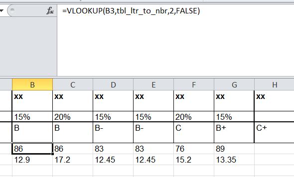
Before getting the letter grade, however, I need to take the letters associated with the individual assignments (cols B-G in row 1) and convert those to numbers. This should go in col N and then col N would be used in a lookup to get the final letter for col O. (The tables for going back and forth are in the sheet “Grade Conversion Tables.”)
However, the formula in col N is not working. The first part makes sure that valid grades have been entered for the 6 assignments. That is working. Given that, the 2nd half starting with the SUMPRODUCT (and I’ve tried many variations including SUM) is supposed to compute the numerical value of the weighted assignment grades. That is not working.
To isolate the 2nd half, I copied/pasted the formula (w/o an equal sign) to cell Q4, deleted the first part of the formula checking for valid grades, and just left the SUMPRODUCT. Still got 0 (answer should be 83.55).
However when I copied/pasted the formula from Q4 to R4, and then converted each “array” (Array 1 is the OFFSET argument to get the numerical equivalents of the letters from the “Grade Conversion Table” sheet; Array 2 is the weights from B2:G2 of the Grades sheet) to numbers using F9 and not hitting ESC to convert back to arguments, I get a valid result.
Moreover, I can see these 2 arrays of values if I highlight the part of the formula in Q4 and hit F9. So Q4 seems to be equivalent to R4 but the results are different.
There are macros in the workbook, which work fine, that will calculate the final grade for col O but I wanted to see if I could do this w/o a macro.
Suggestions?
TIA
Fred

