Time conversion formula using Seconds for macro triggers

Topic

New Reply

I use a process that converts fixed date and time data to total seconds on the time factor only.
The date from the data import is not required.
It uses the 24 hour clock format.

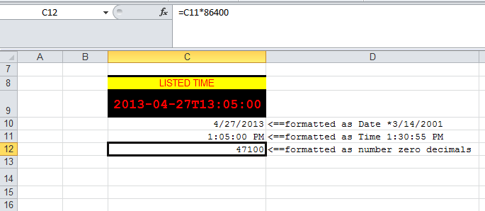
So if data in a cell shows: 25:MAY:2013:10:10:00AM, when it’s split, only the 10:10AM portion is required. This time info is fixed.
This will equate to 36,600 seconds ( past midnight )

The next cell may show 25:MAY:2013:15:38:10
This is the actual computer clock time. This time gets updated with every Do Until Loop.
When calculated it will show 56,280 minutes + 10 seconds = 56,290 total seconds past midnight.
———,

My next formula is subtract 36,600 – 56,290 +(1800) = -17,880
In this case it is a minus sum. It is this Sum I hope to use to trigger a series of macros
The 1800 Seconds is Time zone adjustments
——-,
The following is not essential to trigger the macro, but I’m trying to get the total seconds ( 17,880 back into a read-able look to make other decisions.

When I divide the Total, 17,880.00/60 = 298 minutes
Then divide 298/60 = 4.97

The question is, how do I formulate 4.97 to show the exact hour and minutes PAST 10.10AM when the computer time is 15:38:10 pm ?
I am hoping to achieve -5 Hrs 37 Mins , or whatever the case may be

And,
If it’s before 10:10 am and the computer clock shows 9AM, (32400 seconds), then it’s
36,600 – 32400 + (1800) = 6000 seconds,
6000/60 = 100 minutes ? That can’t be right either, it’s obviously 70 minutes for due time.

Thanks,

Reply | Quote

Replies

Excel can directly add and subtract dates and times (though it does not like negative time!). 15:38:10 (=3:38:10 PM, you are mixing AM/PM with 24-hr clock) – 10:10 AM = 5:28:10 by simple subtraction.

You get 100 mins not 70 mins due to the 1800/60 = 30 mins added by the time zone adjustment. 10:10 AM and 9AM are 70 mins apart when they are in the same time zone. If they are in different timezones it will have to be adjusted.

Steve

Reply | Quote

, ( sorry for the delay, ate something, fish, and still not well)
Thanks for the reply Steve
It is precisely just that, excel does not like negative time, but I need to use the negative to fire one of 3 macro, ( if past this time, then do the next process…etc).
What i have made is a “grid”, has every minute in 24 hours
Example,
Cell F3 has 0:01:00
Cell G3 has a formula, =IF(F3=$A$6,1&”^”,0)
Cell H3 has 60, seconds in 1 minute,
This goes down to half hour blocks

In Cell F22 is 0:30:00
In Cell G22 is my formula, =IF(F32=$A$6,1&”^”,0)
In Cell H22 is ofcourse the 1800, seconds.

If there is a match in Cell A6, or a Vlookup, I then can use the 1800 in this case.

I can then do my subtractions or additions, so when I get those minuses I’m able to work the required macro with variations.
So if I want a macro to fire at 120 seconds prior, it will hopefully fire.
If it’s lets say a negative – 120, it will fire another macro
I am long way from finishing this process, but I hope it works in practice, theory look as though it should?

BTW
I am working with a brand new out of the box office 2010, so it’s going to take a bit of time getting used to all these features.

Reply | Quote

The question is, how do I formulate 4.97 to show the exact hour and minutes PAST 10.10AM when the computer time is 15:38:10 pm ?

XP,

Try the following formula and format the cell C1 as [hh]:mm:ss

A1=36600
B1=56290
C1=ABS((A1-B1)/3600)/24 yields 05:28:10
OR
C1=ABS(5.469444)/24 yields 05:28:10

HTH,
Maud

Reply | Quote

A negative number can be examined by just comparing the values directly. The cell has the negative number in it as a value, whether the display shows what you want or not. If negative, the time formatting does not always work correctly. If that is an issue, you can use ABS (as Maudibe points out) to display it or convert to text that looks like a date in a different cell. There are ways around it.

Not sure what you mean exactly by triggering a macro. There is no event triggered by the calculation of a formula: it does not “change” the cell’s contents… The macro after being triggered can check cells for positive or negative numbers or compare cells to see which is greater…

Steve

Reply | Quote

Thanks maud and Steve;

Try the following formula and format the cell C1 as [hh]:mm:ss

A1=36600
B1=56290
C1=ABS((A1-B1)/3600)/24 yields 05:28:10
OR
C1=ABS(5.469444)/24 yields 05:28:10

HTH,
Maud

I’ll try this and see how it goes,

Not sure what you mean exactly by triggering a macro. There is no event triggered by the calculation of a formula: it does not “change” the cell’s contents… The macro after being triggered can check cells for positive or negative numbers or compare cells to see which is greater…
Steve

Steve,
Maybe it’s my terminology by quoting “triggered”. Activate a macro.
This is what I check for, a Positive within a range or a negative. Therefore 2 possible scenarios to activate 2 If and Then codings.

Reply | Quote

XP,

This code will fire if a calculation was performed on a formula in a cell

Cell C1 contains the formula = A1 – B1

Enter values in A1 or B1. Two different Macros will run conditionally depending if the resulting value in C1 is positive or negative. Entering values in any other cell that is a precedent of another formula yields no fire of either routine A or B on calculation event

Code:

Dim Cell As String

Private Sub Worksheet_Calculate()

If Cell = “$A$1” Or Cell = “$B$1” Then
    If [C1] < 0 Then
        Call RoutineA
    Else:
        Call RoutineB
    End If
End If
End Sub

Private Sub Worksheet_Change(ByVal Target As Range)
    Cell = Target.Address
End Sub

Reply | Quote

Thanks Maud,
I’ll look at that to….

My current “architecture” is to use formula based and a series of 0’s or 1’s
via pre-sets. ( Variables )
A Value in a cell may be 120 Seconds, (+ or -)
I vary that Value to whatever the case may be if required.
This Value in that Cell would be part of the formula If range to get either 1 or 0

What “triggers” the macro would be something like ,

Sub
‘tons and tons of code/formula etc

Do until’s
‘trigger sections

“if cell A7 = 1 then
‘macro xyz
end if
“if cell A8 = 1 then
‘macro ijk
end if

‘more codes/info

Loop

‘The “do nothing and keep Looping because it’s 0
‘Until something changes or becomes 1,

End Sub

That’s the basic idea, for me the 0’s and the 1’s work because of multiple scenarios and quicker
to learn from there, then get into the advanced stages once the logic is sorted, hopefully.

BTW
Still testing other stuff, will get back to this question again, ideas welcomed.

Thanks

Reply | Quote

Just a note of caution, if you are going to have VBA code constantly running in the background to test cell contents, the workbook can get very sluggish and the UNDO feature will not be working (unless you create your own undo feature).

Steve

Reply | Quote

Thanks Steve,
I am aware Excel is not good for repetition, had these problems mainly 2003 version.
2010 version is much better.

The “undo” feature you mention, in this case it’s at the end of a running list of daily-time-order-events.
Up to 12 hours constantly. So when the list becomes empty, it’s the end of the day’s process and End there, hopefully with no glitches.
A dedicated PC is used on the home network for now, the goal is to get to “stand-alone” application once all is sorted.
It has many many times “jammed up” for various reasons and this is where it gets challenging.

But what would be your example of an undo feature, is this some type of VBA code or structure of the entire process ?

XP

Reply | Quote

Hi XP

If you were to describe what you are actually doing, we might be able to give you better alternatives.
For example, perhaps the Excel’s vba ontime process might be appropriate:
Examples:
To run a vba routine myProcedure in 20 seconds time use:
Application.OnTime Now + TimeValue(“00:00:20”), “myProcedure”

To run a vba routine myProcedure at 4:30pm use:
Application.OnTime TimeValue(“16:30:00”), “myProcedure”

To cancel a scheduled process, e.g. to cancel the previous example, use:
Application.OnTime EarliestTime:=TimeValue(“16:30:00″), Procedure:=”myProcedure”, Schedule:=False

So maybe you could avoid some of your problems by scheduling your checks at specific times etc.

zeddy

Reply | Quote

A manual undo feature is code to maintain differences between what is in the book and what is changed. it is relatively complex. The easiest way would be to save backup copies before any change (or major change) and then allow restoring the backup version. Then before closing you could delete any of the temp versions that were saved.

Steve

Reply | Quote

Thanks all,
I will be uploading the workbook in a matter of days, time permitting.

Reply | Quote

Ok,
This Workbook is a Demo, but it’s what really happens.
The timing is critical for it to work right, and it’s basically a workaround because the Web Import, a snippet of info. from a Java countdown Clock does not get Imported. If it did, or when it did it was a number of how much time is remaining to a certain event.
The old VBA used that info to “decide” accordingly.
The Variable method in Seconds is not new either, but was used in Global settings once upon a time when this particular program of mine, ( I had it developed based on my ideas) was actually a server with a script.
Within that script was processes, and these processes used the time factor in seconds. Since then that program data source is obsolete. So it cannot be used anymore, hence I now have to use VBA and not rely on others.
The problem is as stated earlier, Excel does not like to subtract Dates and Times.
So in the Workbook you will a “Grid”. ( Self explanatory)

In Sheets “Settings” is where all the action begins and ends!

In Sheets “Raw Data” is the precise location of the a Date and Time during the Import.
LISTED TIME is static, means when the event will begin out in the real world.

DATA TIME is the time the information of that particular Import was updated.

I also use the PC time in relation to LISTED TIME, but that is not important right now, not there yet.

What I need are the formula in Sheets SETTINGS.

I use 0’s and 1’s based on adding or subtracting Time numerals after I have done a Text Split.
Therefore it’s simple math and Excel does not need to know it’s Time !

Ok
It’s important I get the 0’s and the 1’s to work right within this real time “logic”.

In Sheets, SETTINGS.
Ranges A9 to A11 are 3 basic Variable numeric settings signifying Seconds.

A9 is the first task at 120 seconds before the Listed Time, If the web import arrived in time!
Meaning I may have missed an event, ( happens occasionally) but have allowed a buffer of
59 seconds. ( 120 – 59 = 61 Seconds )
Therefore if my web import is within that range, it is suppose to show a 1. Before 120 or after 61 it is suppose to show 0

However,
In Cell A10, I have 60 Seconds with a buffer of 45. ( 60 – 45 = 15 Seconds )
Within that range I need the formula to show 1, if A9 is 0 after 61

Then
in Cell A11 is 900.
This means the macro has Occured from the 1 in A10 and I can wait for no more that 900 seconds after the event has started.
After the maximum wait ( 900 seconds ) from that time, it must show 1.
1 will then mean, “waited too long for certain data AFTER the event has started, therefore get the next event on a Time order daily event list.

So it’s the formula I need for the above scenarios.

In Sheets TEST SCENARIOS, I put that there to help anyone with some idea of what’s going on.

Thanks

PS
If you are confused, so am I !

Reply | Quote

XP,

You have painstakingly imported a date/time that has an improper format, split it apart into individual components, pieced the time aspects back together into a string, converted the string back to a time format, then converted it into seconds using a lookup table. You have obviously placed a tremendous amount of thought and work in to this project! But there may be an easier approach.

Consider the following routine that could replace your 4 macros (50+ lines of code) and your Time grid:

Code:

Public Sub SplitDate()
Dim s As Variant
s = Split([C9], “T”)
[c10] = s(0)  ‘DATE
[c11] = s(1)  ‘TIME
End Sub

34406-xp

The 86400 comes from 60 sec/min * 60 min/hr * 24 hrs/day. From our past discussions, it is kind of neat to see your application come to light.

HTH,
Maud

Reply | Quote

Thanks Maud,
I knew there is a simpler way.. and once the entire process is “joined”, then the code_culling begins.

I appreciate everyone’s help.

But for now I have to get those formula working right and use the 0’s and the 1’s.
Once that logic is sorted, then yes, I will be able to concentrate on what Private Subs and Dims are all about. I don’t “see” it any other way.

The overall architecture ?
Yes, That I know what needs to be done.

Thanks.

Reply | Quote

XP,

I played with the XML code of the web sheet and finally got it working. The problem was on how they format the name of the xml file in relation to the url. Once I figured that out, The code ran flawlessly. Here was its output.

34431-xml-code

Does any of this data offer any help?

Maud

Reply | Quote

It looks neat, I’ve seen XML imports before.

The example workbook is an import by using first a recorded web query macro, then tweaking the code thereafter.

In sheet1 you will see some clutter, this is the “raw” Inoprt.
In sheet 2 is what it looks like after a macro cleans it up.
I use most or all of that information and make mathematical calculations and strategies.

Once that even has ended, the same event will show Results of that event.
That information is used to, IF the event suited the criteria from those calculations.

In any case, the countdown timer’s information, ( a numeral ) does not seem to get imported.
That’s the whole purpose of this phase.
In sheet2 cell C9 is 2013-07-21T12:10:00 the start time of the event
in cell D24 2013-07-21T11:50:15 is the time of that updated information.

My variables for the Time factor are calculated From Seconds.
So in Sheet 3 for example, if I choose 120 and I get a Match from the time grid I made, then the macro makes it’s “decisions” accordingly, (100% hands free).
The goal of the learning curve to learn VBA is to eliminate EVERY mouse click.

Hope this helps.

The Tables used after the tweak

Code:

‘[B] & Range (“A2”)[/B] means the url reference is constructed as :[B]2013/3/31/BS/1[/B]
On Error GoTo notfound ‘
    With ActiveSheet.QueryTables.Add(Connection:= _
        “URL;http://tatts.com/racing/” & Range(“A2”), Destination:=Range(“$A$3”))
        ‘2013/3/31/BS/1
        .FieldNames = True
        .RowNumbers = False
        .FillAdjacentFormulas = False
        .PreserveFormatting = True
        .RefreshOnFileOpen = False
        .BackgroundQuery = True
        .RefreshStyle = xlOverwriteCells
        .SaveData = True
        .AdjustColumnWidth = True
        .RefreshPeriod = 0
        .WebSelectionType = xlSpecifiedTables
        .WebFormatting = xlWebFormattingNone
        .WebTables = “1,2,3,4,5,6,7,8,10,11,12,13,””pooldata””,55″
        .WebConsecutiveDelimitersAsOne = True
        .WebSingleBlockTextImport = False
        .WebDisableDateRecognition = False
        .WebDisableRedirections = False
        .Refresh BackgroundQuery:=False

Reply | Quote

XP,

The following code will copy the entire web page to a sheet in a similar fashion to a web query but not limited to just tables. For the particular webpage that you are using, the field that contains the data you seek is consistently placed in Cell D21. You could download the data to a hidden sheet at insertion point cell A1. NOTE: It takes several seconds for the download.

Using my code above, the mal-formatted Date/Time (D21) is split and the countdown minutes are calculated (Start time minus system time). The calculated countdown (in minutes) can be placed directly into the cell that requires the number.

HTH,
Maud

Code:

Sub ReadWebPage()
[COLOR=”#008000″]’DECLARE AND SET VARIABLES[/COLOR]
Dim webpage As String
Dim insertion As Range
webpage = “http://google.com”  [COLOR=”#008000″]’CHANGE TO CORRECT URL[/COLOR]
Set insertion = Worksheets(“Sheet2”).Range(“$A$1″) [COLOR=”#008000”] ‘CHANGE DESTINATION INSERTION POINT[/COLOR]
[COLOR=”#008000″]’————————————————————————-
‘DOWNLOAD WEB PAGE[/COLOR]
With Worksheets(“Sheet2”).QueryTables.Add(Connection:= _
    “URL;” & webpage, Destination:=insertion)
    .WebSelectionType = xlEntirePage
    .Refresh BackgroundQuery:=False
End With
[COLOR=”#008000″]’———————————————————————————
‘CALCULATE THE REMAINING MINUTES[/COLOR]
With Worksheets(“Sheet2”)
s = Split(.Range(“D21”).Value, “T”)
.Range(“H23″).Value = Minute(s(1)) – Minute(Time())  [COLOR=”#008000”]’CHANGE TO CELL THAT REQUIRES COUNTDOWN[/COLOR]
End With
End Sub

Reply | Quote